Every article that has ever given advice on investing in venture capital has said that you need to invest in a portfolio of companies, because each investment on its own is probably going to be worth nothing and if you invest in just a few you will almost certainly lose all your money. This is good advice.
If you want to know exactly how much to diversify, that’s a harder question. There are a lot of articles and posts out there that give you advice on how big your angel portfolio should be. I think they’re wrong. Maybe not in the advice they give, but in their methodology. They are a dead end.
Every person in venture, when pushed on why either so many companies don’t succeed or on why any young company deserves to be valued at $1 billion or more, says that it’s because venture-backed companies follow a power law. But when they think about portfolio construction, they treat outcomes as some other sort of distribution, one that’s easier to reason about. This post will take the hard road and try to reason about power law distributions. That means math, and code.
Portfolios in the Normal World
First, a thought experiment. Let’s say someone gives you a die and tells you that if you roll a six you win twelve dollars for every dollar you bet, otherwise you lose: you bet $100. If you roll a 1, 2, 3, 4, or 5 you lose your $100; if you roll 6 you get $1200. It’s a good bet for you: you end up with nothing five-sixths of the time but with $1200 one-sixth of the time. Your expected value is $200, double your bet.
Now the person you are wagering against asks you to divvy up your $100 into some number of equal bets. How many bets should you make?
On the one hand, whether you make 1 bet or 1000 bets, the expected value remains the same: $200. But if you make one bet, you will probably lose your entire bankroll, with a small chance of multiplying it twelvefold. If you make 1000 bets, you will almost certainly end up with exactly twice your bankroll. This is just the Law of Large Numbers: the average of a sample tends to approach the expected value as the size of the sample increases: the more bets you make, the more your average outcome looks like the average of the distribution itself. The standard deviation of the outcome gets smaller and the probability of results far from the expected value decreases.


I simulated this in code. The first chart is a simulation where you bet $5 on each of twenty rolls. The second chart is where you bet $0.50 on each of 200 rolls. I ran each simulation 10,000 times and plotted the distribution of outcomes.
If you look at the first chart, it shows you end up with less than you started with more than 10% of the time. You most often end up with around $200, of course, but there’s an excellent chance you end up with more than $300.
When you divvy your bankroll into 200 parts—the second chart—you almost never lose money.1 But you also almost never make more than $300. Your outcome of your portfolio of bets is more predictable when you make more of them.
This is the the entirety of the content of the advice that you should have a lot of companies in your venture capital portfolio: you have a lower chance of losing money the more companies you invest in. Of course, by the same reasoning you also have a lower chance of making a lot of money, although the people giving the advice rarely highlight that part. A ton of bets is the right way to match the market return with this sort of distribution of outcomes—distributions with a finite mean and variance, including all distributions with a finite number of possible outcomes (like rolling a die) as well as common distributions like the normal distribution and the lognormal distribution.
Monte Carlo Simulations
Venture capital is more complicated than throwing a die. There are not only more than six possible outcomes, there are, at least, billions of possible outcomes. The example with the die could have been calculated fairly simply: it’s a textbook binomial distribution. But when you have a lot of outcomes it’s easier to have a computer simulate picking samples from a distribution and take averages over thousands of simulated portfolios. This process is generally called a Monte Carlo Simulation.
As an example, let’s take the very high-level distribution of venture returns from Fred Wilson’s 2012 blog post, The Power of Diversification: “the average startup has a 33% chance of making money for the investors, a 33% chance of returning capital, and a 33% chance of losing everything and that only 10% will make a big return (>10x).” The actual model he uses in the post is slightly different, here it is:
\[\begin{align*}p(x)=\left\{
\begin{array}{l}
Pr(X=0) &= 40\% \\
Pr(X=1) &= 30\% \\
Pr(X=3) &= 20\% \\
Pr(X=10) &= 10\% \\
\end{array}
\right.
\end{align*}\]
There’s a 40% chance any single company returns nothing, a 30% chance it returns what you invested, a 20% chance it returns three times what you invested, and a 10% chance it returns ten times. Call this the Basic Model. Note that its expected value is \(30\%*1 + 20\%*3 + 10\%*10=1.9\).
To Monte Carlo simulate the Basic Model you would choose a portfolio size, n, pick n outcomes from the distribution, and take the average of those n picks. This is the outcome of one random portfolio. Do this thousands of times and chart the distribution of averages. Then vary n to find the distribution of averages for different portfolio sizes.
Below is Python 2.7 code using numpy and pyplot to simulate the Basic Model.
This file contains bidirectional Unicode text that may be interpreted or compiled differently than what appears below. To review, open the file in an editor that reveals hidden Unicode characters.
Learn more about bidirectional Unicode characters
| import numpy as np | |
| def pickaportfolio(n): | |
| # possible outcomes, from Fred's post | |
| # portfolios of size n | |
| # returns the mean of a single random portfolio | |
| possible_outcomes = [0,0,0,0,1,1,1,3,3,10] | |
| # pick n random elements from the list and take the mean of the outcome | |
| return np.mean(np.random.choice(possible_outcomes,n)) | |
| def lotsofportfolios(m,n): | |
| # m portfolios of n picks each | |
| # returns a list of m means of portfolio size n | |
| return [pickaportfolio(n) for _ in range(m)] | |
| def chartports(n): | |
| # Plot 10,000 runs with portfolio size n | |
| # no return value, chart is side-effect | |
| portfolios = lotsofportfolios(10000,n) | |
| plt.title('Distribution of returns, portfolio size %d' % n) | |
| tallest=max(plt.hist(portfolios,bins=[0,1,2,3,4,5,6,7,8], rwidth=0.7,align='mid')[0]) | |
| plt.grid(True) | |
| plt.xlabel('Portfolio Return Multiple') | |
| plt.yticks(np.arange(0,tallest-tallest%-len(portfolios)/10.,len(portfolios)/10.), | |
| ('0%','10%','20%','30%','40%','50%','60%','70%','80%','90%','100%') ) | |
| plt.show() | |
| print "Mean = %.3f" % np.mean(portfolios) |
Here are several runs with different portfolio sizes.
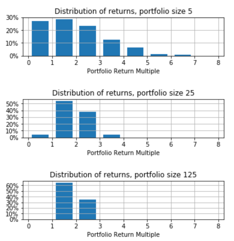
As with the die example, the larger the portfolio, the less variance from the expected value, 1.9.
Fred’s post says: “If you make just one investment, you are likely going to lose everything. If you make two, you are still likely to lose money. If you make five, you might get all your money back across all five investments. If you make ten, you might start making money on the aggregate set of investments.” The below runs of the model show what he means.
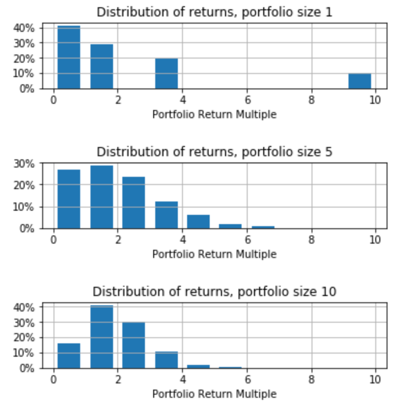
If your portfolio size is 1, you lose everything 40% of the time. You make money 30% of the time. And you get your money back 30% of the time. As the portfolio size grows, your chance of losing money shrinks and your chance of making money grows. (The average stays the same.)
| Portfolio Size | Percent <=1x | Percent >1x | Mean |
| 1 | 70% | 30% | 1.9x |
| 5 | 35% | 65% | 1.9x |
| 10 | 20% | 80% | 1.9x |
This example doesn’t allow for the small probability of a single company returning more than 10x. This would make sense if extreme outcomes are extremely unlikely and not really that far from the mean. Bucketing them into a catch-all like 10x is accurate enough (and, in the pedagogic sense Fred is embracing, anything above 10x is gravy; better to be conservative when giving advice to amateurs.)
This model not only answers “how many companies should be in my portfolio so that I have less than a 10% chance of losing money?”, it shows you that as you make more investments in a portfolio, you are taking less risk. The average will always be close to 1.9x, even with small portfolios, but the variability (or risk) will shrink as the portfolio size grows. This is just the law of large numbers at work. But the law of large numbers does not work with fat-tailed distributions.
Fat-tailed Distributions
All of these Monte Carlo simulations have one crucial problem: the full range of possible outcomes is much, much larger than the sample the simulation draws from. This is obvious in the Basic Model, where there are only four possible outcomes.2 It’s less obvious when the set of possible outcomes is much larger.
Many of the articles that recommend a minimum portfolio size for early stage investors use data from real investing outcomes. (Here are some posts using data from the Angel Investor Portfolio Project that the Kauffman Center ran: link, link, link, link, link. I believe this one relies on the same data, but I’m not positive.) The AIPP collected actual outcomes on 1,137 angel investments over many years.3
The relative strengths of using AIPP dataset is that there is no bucketing—each possible outcome is an actual outcome—and the large number of outcomes represented. Monte Carlo Simulations using the data pick portfolios from these 1,137 outcomes. The implicit argument is that the outcomes that are not in the AIPP data must be not very different from the ones that are, because the sample is so large, and that any real outliers are so unlikely that their expected value doesn’t change the average outcome much at all.
But is this true?
Take the AIPP, with it’s average outcome of 2.43x (after the data is cleaned.) Then add in a few outcomes that weren’t in their data: a 10,000x (estimate of Google seed multiple), a 5000x (estimate of Uber seed multiple), and a 3000x (estimate of WhatsApp seed multiple). If you add these the average of the distribution increases from 2.43x to more than 18x. This is hardly fair because I’m cherry-picking, but you see the point: the extremely unlikely tail of the venture capital outcome distribution contributes a meaningful amount to the mean outcome.4 This is the “fat tail” or “black swan” outcome talked about by Taleb in his popular book. With some assumptions, we can quantify it.
Assumption 1: The outcomes of venture capital investments are power-law distributed. Here we’ll talk about outcomes as multiples of amount invested (ie. 1x, 2x, etc.) I talk about power-law distributions (PLDs) in venture in a previous post, which is probably worth reading. A PLD is of the form \(p(x) = Cx^{-\alpha}\), where the normalization constant \(C = (\alpha – 1)x_0^{\alpha-1}\), with \(x_0\) the minimum value x can take.
Assumption 2: The actual distribution of outcomes has an alpha of something just below 2. We will use \(\alpha = 1.98\). There’s evidence for this in the previous post I just mentioned.
Assumption 3: This is the tricky one.
We need to adjust the vanilla PLD to account for the 1/3=0x, 1/3=1x piece. A PLD can’t ever have a value for zero (it would be infinite, and the area of a distribution has to sum to one) so there has to be a dynamic that distorts the underlying PLD at the low end. This may be due to (a) the cost of unwinding a failing company (if a company is worth less than, say, 50% of what was put in, the cost of unwinding it means no money at all is returned); and (b) the structure of venture contracts (preferred stock, convertible loans) that return value to the investors first (if a company is worth 80% of the money put in, the venture investors are made whole first, so they probably get 1x.)
We could adjust the PLD to set \(x_0\) such that 2/3 of the weight of the distribution falls below 1 and then transform the first third of the weight to zero and the second third to one, leaving the rest as is. But since a PLD is self-similar, we will do something simpler:
\[\begin{align*}p(x)=\left\{
\begin{array}{l}
Pr(X=0) &= 1/3 \\
Pr(X=1) &= 1/3 \\
Pr(X=x) &= \frac{1}{3}Cx^{-\alpha}, x>1 \\[10pt]
\end{array}
\right.
\end{align*}\]
In this case, \(x_0\) is 1, but \(\alpha\) stays the same.
Those are the assumptions, and the question is: given a finite set of possible outcomes, how well do they represent the actual distribution?
Any set of possible outcomes misses out on all the possible outcomes larger than the largest in the set, so we can reframe the question as: how much of the mean of the distribution comes from the tail, the part of the distribution further along the x-axis than the largest value in our sample? How fat is the tail? More concretely, if we are using the AIPP data, where the best outcome was 1333x, how much of the mean comes from outcomes larger than that?
To figure this out, we will segment the probability distribution into two pieces: the base and the tail, and note that the mean of the distribution is the mean of the base plus the mean of the tail [EDIT: I should have said the contribution of the base to the mean plus the contribution of the tail to the mean equals the mean]. This sounds funny, so an example.
You throw a die. You have a 1/6th chance of throwing any number 1 through six. The mean outcome is (1+2+3+4+5+6)/6=3.5. Now define throwing 1 or 2 as the base and throwing 3 through 6 as the tail. The mean of the base is (1+2)/6=0.5 and the mean of the tail is (3+4+5+6)/6=3.0. The sum of these is the mean of the distribution. It’s the same for a PLD but because a PLD is continuous, not discrete, we’re going to have to use calculus.
The mean of a probability distribution is
\[<x> =\displaystyle\int xp(x)\,dx\]so the mean of a PLD is
\[<x> =\displaystyle\int_{x_0}^\infty xCx^{-\alpha}\,dx =C\int_{x_0}^\infty x^{-\alpha+1}\,dx = \left[C\frac{x^{2-\alpha}}{2-\alpha}\right]_{x_0}^\infty\]For our distribution \(x_0 = 1\), so \(C = \alpha-1\):
\[<x> =\left[(\alpha-1)\frac{x^{2-\alpha}}{2-\alpha}\right]_1^\infty = 0\, – \frac{\alpha-1}{2-\alpha} = \frac{\alpha-1}{\alpha-2}\]Note that this mean makes no sense when \(\alpha<2\). Going back to the indefinite integral you can see that the mean of a PLD with \(\alpha<2\) is infinite.
To compare the mean of the base and the mean of the tail of a PLD, we’ll pick an arbitrary division between the two and call it b.
\[<x> = \displaystyle\int_1^\infty xCx^{-\alpha}\,dx = \int_1^bxCx^{-\alpha}\,dx + \int_b^\infty xCx^{-\alpha}\,dx =<x_{base}> + <x_{tail}>\]The first term is the mean of the PLD up to b, the base, and the second term is the mean of the tail.
\[<x> =\left[\frac{\alpha-1}{2-\alpha}x^{2-\alpha}\right]_1^b+\left[\frac{\alpha-1}{2-\alpha}x^{2-\alpha}\right]_b^\infty = \frac{\alpha-1}{\alpha-2}\left(1-b^{2-\alpha}\right)+\frac{\alpha-1}{\alpha-2}b^{2-\alpha}\]So
\[<x_{base}> = \frac{\alpha-1}{\alpha-2}\left(1-b^{2-\alpha}\right)\]and
\[<x_{tail}> =\frac{\alpha-1}{\alpha-2}b^{2-\alpha}\]Using this, if we know the mean of the base we can figure out how much bigger the mean of the entire distribution is: \(\frac{<x>}{<x_{base}>}\).
From above, \(<x>= \frac{\alpha-1}{\alpha-2}\) so
\[\begin{align}\frac{<x>}{<x_{base}>} &=\frac{\frac{\alpha-1}{\alpha-2}}{\frac{\alpha-1}{\alpha-2}\left(1-b^{2-\alpha}\right)} \\
&=\frac{1}{1-b^{-(\alpha-2)}}
\end{align}\]
Note that if alpha is greater than 2 then \(b^{-(\alpha-2)}\) is less than one and so this fraction is greater than one: the mean of the distribution is greater than just the part contributed by the base. We knew that. But as alpha gets close to 2, \(b^{-(\alpha-2)}\) gets close to 1 and the fraction gets very large. As alpha approaches 2, more and more of the distribution’s mean is contributed by the tail until at 2 or lower, all of it is.
Let’s use the AIPP data as an example. The base of the distribution is all the outcomes in the data set, while the tail will be all the outcomes larger than the largest outcome in the dataset. How well does the mean of the AIPP outcomes reflect the mean of the distribution?
The dividing line between base and tail, b, is the largest outcome in the dataset: 1,333 times the initial investment. The mean of the AIPP dataset is 2.43x. This is the mean of the whole distribution including 0s and 1s, call it \(<x^\prime_{base}>\). To get from this to the mean of just the power law part, \(<x_{base}>\), back out the other parts:
\[<x^\prime_{base}>=\frac{0}{3}+\frac{1}{3}+\frac{<x_{base}>}{3}\]so
\[<x_{base}>=3<x^\prime_{base}>-1=6.29\]and the mean of the part of the distribution greater than 1 is
\[\begin{align}{<x>} &= \left(\frac{<x>}{<x_{base}>}\right){<x_{base}>} \\
&=\left(\frac{1}{1-b^{-(\alpha-2)}}\right)<x_{base}> \\
&=\left(\frac{1}{1-1333^{-(\alpha-2)}}\right)6.29
\end{align}\]
and the mean of the entire implied underlying distribution, including 0s, 1s, and the power law tail not in the outcome is \(<x^\prime>=\frac{2.1}{1-1333^{-(\alpha-2)}}+\frac{1}{3}\).
Here is a chart of the results for alphas between 2 and 2.25.

You can see that as alpha gets large, \(\frac{<x>}{<x_{base}>}\) gets closer to one and the mean of the total distribution is the same as the mean of the dataset. Since a large alpha means a short tail this makes sense. If the tail is short then most of the weight of the distribution is in the base. But as alpha approaches two, this mean of the underlying distribution gets larger and larger: more and more of the mean is in the tail. At two, it becomes infinite.
When the alpha of the distribution is 2.1 the mean of the actual underlying distribution is about 1.8 times the mean of the sample (the sample is the AIPP data). When the alpha=2.05 the actual mean is three times the sample mean. When the alpha is 2.01 the actual mean is more than 30. At alphas close to 2, the sample data misrepresents the underlying distribution by a huge amount. If alphas are less than 2.1, any Monte Carlo Simulation using the AIPP data does not represent the actual underlying distribution in any meaningful way. You can’t use the Monte Carlo Method to simulate a fat-tailed distribution, it won’t be accurate.
One final kicker. It seems like the alpha of venture capital outcomes is less than 2, in the 1.9-2.0 range. If so, the ratio of the mean of the distribution to the part contributed by the base is infinite. In the venture world, the average of any set of sample outcomes, no matter how large, does not represent the mean of the total distribution. Using a sample, even a really big sample, even a sample that has the return of every venture investment in history, to create a Monte Carlo Simulation is the wrong way to analyze venture outcomes.
You can’t simulate venture portfolios using a sample dataset, you have to use the underlying distribution from which the data are presumably drawn, a power law distribution with a fat tail, an \(\alpha\) just less than 2.
Using Power Law Distributions to Simulate Venture Portfolios
A PLD with a fat tail like this can be hard to work with. The mean is infinite, so some of the analyses we would like to do just result in infinity, which is hard to reason about. After all, the next company you invest in is not going to be worth infinity. The variance is also infinite, so Monte Carlo Simulations are unstable, because outliers big enough to skew even a 10,000 iteration run pop up.
The most helpful thing to know would be the average return of a portfolio with a confidence interval. If you have a portfolio size n, then the average return is m +/- 5% with probability 95%, that sort of thing. This is not possible to calculate in venture because the law of large numbers does not hold when the mean of the distribution is not finite.
Since the mean of the distribution is infinite, the average mean across all possible portfolios of any given size is also infinite. Of course, any actual sample from the distribution will consist of finite numbers with a finite average. But will increasing your portfolio by one more company increase or decrease the average of the entire portfolio?
Assuming the existing average is greater than one, then most of the time the next pick will decrease the average (because two thirds of the distribution is one or less so at least two thirds of the distribution has a lower value than your current average.) But in the less likely case that the new entry into your portfolio is larger than the current average, it will be on average extremely large. So while each new company in the portfolio will most likely lower your average return, when it doesn’t it increases the average by a lot. This isn’t two steps forward, one step back, it’s one step back, one step back, one step back, ten steps forward.
If this is so your portfolio should be as large as you can make it (so long as you can keep your alpha below 2.)
So if we can’t calculate that, what can we calculate? The most helpful analysis I can run is the probability of a portfolio of a given size exceeding a benchmark return, one times the money invested, two times the money invested, three times the money invested, etc.
If the portfolio has one company, this is easy. Imagine your portfolio size is one: what is the probability of a return greater than or equal to 1x? Given our probability distribution (1/3 0x, 1/3 1x, 1/3 greater than one) we know the answer is 2/3.
If the portfolio is size two, the answer can still be calculated using probability. Each of 0x, 1x, and the power law distribution that is greater than 1x is equally likely. So there are nine equally likely possible outcomes:
| 1. (0,0) < 1 |
| 2. (0,1) < 1 |
| 3. (1,0) < 1 |
| 4. (1,1) = 1 |
| 5. (0,>1) = ? |
| 6. (>1,0) = ? |
| 7. (1,>1) > 1 |
| 8. (>1,1) > 1 |
| 9. (>1,>1) > 1 |
1, 2, and 3 are less than 1x. 4, 7, 8, and 9 are greater than or equal to 1x. 5 and 6 could be either: if the >1 part is greater than or equal to 2 then the average will be greater than or equal to 1. The 1x part is greater than 2 with probability
\[P(x>2)=C\int_2^{\infty}x^{-\alpha}\,dx=2^{-\alpha+1}\]
If \(\alpha=1.98\) then P(x>2)=51%. So a two company portfolio equals or exceeds 1x when it is (1,1), (1,>1), (>1,1), (>1,>1) and 50.7% of the time when it is (0,>1) or (>1,0). This is 4/9 + (2/9)*50.7% = 55.7% of the time. This reasoning could theoretically be continued for any size portfolio but it would quickly become super-complicated, so we’re going to use a Monte Carlo Simulation. Unlike the AIPP Monte Carlos, this Monte Carlo is not going to pick from an existing set of data, it will pick from the distribution.
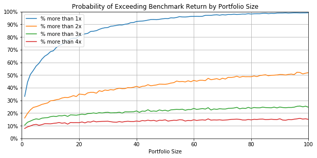
I charted the percentage of portfolios exceeding 1x, 2x, 3x, and 4x by size of portfolio, with alpha=1.98 (The code is below.) To exceed one times your investment (that is, make money) 90% of the time, you need a portfolio of at least 34 companies. To exceed 2x 50% of the time, you need a portfolio of at least 85 companies.
Here is the code.
This file contains bidirectional Unicode text that may be interpreted or compiled differently than what appears below. To review, open the file in an editor that reveals hidden Unicode characters.
Learn more about bidirectional Unicode characters
| import numpy as np | |
| def vcdist(alpha): | |
| # generates one pick from the VC distribution | |
| # prob density distribution = 1/3 0x, 1/3 1x, 1/3 power law with alpha=alpha | |
| # returns one draw from the distribution as a float | |
| pn=np.random.randint(0,3) | |
| if pn==2: | |
| td = powerlaw.Power_Law(xmin=1.0, parameters=[alpha]) | |
| return td.generate_random(1)[0] | |
| return pn | |
| def vcportfolios(alpha,n): | |
| # creates 10,000 random portfolios, each of size n and finds average mean | |
| # of those portfolios and the percent of those portfolios above 1x,2x,3x,4x | |
| # returns tuple: (mean, %>1x, %>2x, %>3x, %>4x) | |
| runs=10000. | |
| portfolioavgs=[average([vcdist(alpha) for i in range(n)]) for j in range(int(runs))] | |
| return (average(portfolioavgs), | |
| (len([i for i in portfolioavgs if i>1.])/runs), | |
| (len([i for i in portfolioavgs if i>2.])/runs), | |
| (len([i for i in portfolioavgs if i>3.])/runs), | |
| (len([i for i in portfolioavgs if i>4.])/runs)) | |
| def plt_vcports(alpha): | |
| # runs vcportfolios at portfolio sizes from 1 to 100 | |
| # charts result | |
| # no return value | |
| xm,xm1,xm2,xm3,xm4=[],[],[],[],[] | |
| X=range(1,101,1) | |
| for i in X: | |
| m,m1,m2,m3,m4 = vcportfolios(alpha,i) | |
| xm.append(m) #mean, not charted here | |
| xm1.append(m1) #more than 1x | |
| xm2.append(m2) #more than 2x | |
| xm3.append(m3) #more than 3x | |
| xm4.append(m4) #more than 4x | |
| # chart results | |
| ax = plt.figure(figsize=(10, 10)).add_subplot(211) | |
| ax.plot(X,xm1,X,xm2,X,xm3,X,xm4) | |
| ax.set(xlim=[0, 100], ylim=[0,1], | |
| title='Probability of Exceeding Benchmark Return by Portfolio Size', | |
| xlabel='Portfolio Size', yticks=np.arange(0,1.1,.1)) | |
| ax.yaxis.set_major_formatter(FuncFormatter(lambda y, _: '{:.0%}'.format(y))) | |
| ax.grid(True) | |
| ax.legend( ('% more than 1x','% more than 2x','% more than 3x','% more than 4x'),loc='upper left') |
That’s looking at how many companies you need to reach some probability of exceeding some metric. You can also assume a fixed portfolio size and calculate the probability that it exceeds each benchmark. In the chart, if you have a portfolio of 40 companies, you will meet or exceed 1x 92% of the time, 2x 44% of the time, 3x 24% of the time, and 4x 16% of the time. An easier way to look at this is to make a table of outcomes, and I’ve done that, below.
Here’s the code to generate the percent above the first 15 benchmarks (>=1x, >=2x, …>=15x) for a given portfolio size. It runs somewhat faster than the code above, although I’m sure it could be optimized further.
This file contains bidirectional Unicode text that may be interpreted or compiled differently than what appears below. To review, open the file in an editor that reveals hidden Unicode characters.
Learn more about bidirectional Unicode characters
| import numpy as np | |
| def vcdraws(alpha,n): | |
| # prob density distribution = 1/3 0x, 1/3 1x, 1/3 power law with alpha=alpha | |
| # returns list of n draws from the distribution | |
| pn=np.random.randint(0,3, size=n) | |
| td = powerlaw.Power_Law(xmin=1.0, parameters=[alpha]) | |
| return [td.generate_random(1)[0] if pn[i]==2 else pn[i] for i in range(n)] | |
| def vcportdraws(alpha,portsize,runs): | |
| # generate runs portfolios of size portsize | |
| # returns % of portfolios whose average is above 1..15 in 15-item list | |
| numd=portsize*runs | |
| ports = vcdraws(alpha,numd) | |
| avgs = [average(ports[i:i+portsize]) for i in range(0,numd,portsize)] | |
| count=[0,0,0,0,0,0,0,0,0,0,0,0,0,0,0] | |
| inc = 1./runs | |
| for i in avgs: | |
| for j in range(15): | |
| if i>(j+1): count[j]+=inc | |
| return [int(i*1000)/10. for i in count] |
And here is the table.
| % of portfolios that equal or exceed multiple | |||||||||||||||
|---|---|---|---|---|---|---|---|---|---|---|---|---|---|---|---|
| Port. Size | 1x | 2x | 3x | 4x | 5x | 6x | 7x | 8x | 9x | 10x | 11x | 12x | 13x | 14x | 15x |
| 1 | 33.2 | 16.6 | 11.2 | 8.7 | 6.9 | 5.8 | 4.9 | 4.2 | 3.8 | 3.4 | 3.1 | 2.9 | 2.7 | 2.5 | 2.3 |
| 2 | 55.5 | 20.7 | 13.8 | 10.4 | 8.0 | 6.5 | 5.3 | 4.8 | 4.1 | 3.8 | 3.3 | 3.0 | 2.7 | 2.6 | 2.3 |
| 5 | 56.8 | 24.4 | 15.2 | 10.8 | 8.5 | 6.8 | 5.8 | 4.8 | 4.3 | 3.9 | 3.5 | 3.3 | 3.0 | 2.8 | 2.6 |
| 10 | 67.8 | 29.3 | 17.2 | 11.7 | 9.0 | 7.3 | 6.0 | 5.1 | 4.6 | 4.1 | 3.7 | 3.4 | 3.0 | 2.8 | 2.6 |
| 20 | 80.0 | 34.3 | 19.1 | 12.6 | 9.3 | 7.4 | 5.9 | 5.0 | 4.3 | 3.8 | 3.4 | 3.0 | 2.7 | 2.5 | 2.3 |
| 30 | 87.8 | 41.2 | 23.0 | 15.0 | 10.8 | 8.5 | 7.2 | 6.1 | 5.3 | 4.6 | 4.2 | 3.7 | 3.5 | 3.1 | 3.0 |
| 40 | 92.4 | 43.9 | 23.6 | 15.5 | 11.4 | 8.9 | 7.2 | 6.1 | 5.3 | 4.6 | 3.6 | 3.2 | 3.0 | 2.7 | 2.6 |
| 50 | 94.9 | 46.9 | 24.8 | 15.9 | 11.4 | 9.0 | 7.1 | 5.9 | 5.3 | 4.6 | 3.9 | 3.6 | 3.2 | 2.9 | 2.6 |
| 60 | 96.7 | 48.9 | 25.3 | 15.8 | 11.7 | 9.2 | 7.4 | 6.3 | 5.4 | 4.8 | 3.7 | 3.4 | 3.0 | 2.9 | 2.6 |
| 70 | 97.8 | 50.6 | 26.4 | 17.0 | 12.5 | 9.4 | 7.8 | 6.5 | 5.5 | 4.9 | 3.8 | 3.4 | 3.1 | 2.9 | 2.6 |
| 80 | 98.6 | 53.6 | 27.7 | 17.4 | 12.5 | 9.8 | 7.9 | 6.6 | 5.8 | 5.1 | 3.8 | 3.4 | 3.1 | 2.8 | 2.5 |
| 90 | 99.0 | 54.8 | 28.7 | 18.2 | 12.9 | 10.0 | 8.2 | 7.0 | 6.0 | 5.2 | 4.0 | 3.6 | 3.3 | 3.0 | 2.7 |
| 100 | 99.3 | 56.8 | 29.7 | 18.6 | 13.2 | 10.2 | 8.2 | 6.9 | 5.9 | 5.2 | 3.9 | 3.5 | 3.0 | 2.8 | 2.6 |
| 200 | 99.9 | 69.0 | 34.8 | 20.9 | 14.0 | 10.8 | 8.9 | 7.4 | 6.1 | 5.3 | 4.7 | 4.1 | 3.6 | 3.4 | 3.1 |
| 300 | 99.9 | 76.3 | 38.3 | 22.5 | 15.1 | 11.3 | 9.1 | 7.4 | 6.3 | 5.5 | 5.3 | 4.9 | 4.3 | 4.0 | 3.6 |
| 400 | 99.9 | 81.4 | 41.7 | 24.0 | 16.0 | 11.9 | 9.5 | 7.7 | 6.5 | 5.8 | 5.1 | 4.6 | 4.0 | 3.7 | 3.4 |
| 500 | 99.9 | 85.5 | 43.1 | 24.4 | 16.6 | 12.1 | 9.5 | 7.7 | 6.3 | 5.3 | 5.1 | 4.7 | 4.2 | 3.8 | 3.5 |
| 600 | 99.9 | 88.6 | 45.6 | 25.4 | 16.8 | 12.2 | 9.4 | 7.8 | 6.6 | 5.6 | 5.4 | 4.9 | 4.5 | 4.0 | 3.6 |
| 700 | 99.9 | 90.7 | 47.4 | 26.5 | 17.3 | 12.5 | 10.1 | 8.2 | 6.9 | 5.8 | 5.1 | 4.6 | 4.1 | 3.7 | 3.5 |
| 800 | 99.9 | 92.7 | 49.2 | 26.9 | 17.6 | 12.8 | 10.1 | 8.0 | 6.7 | 5.7 | 5.4 | 4.8 | 4.4 | 4.0 | 3.8 |
| 900 | 99.9 | 93.8 | 49.9 | 27.5 | 17.6 | 12.7 | 9.7 | 7.9 | 6.7 | 5.7 | 5.3 | 4.6 | 4.1 | 3.7 | 3.4 |
| 1000 | 99.9 | 94.9 | 52.1 | 28.1 | 18.1 | 13.1 | 10.3 | 8.3 | 6.9 | 5.8 | 5.5 | 5.0 | 4.5 | 4.1 | 3.6 |
| 10,000 | 100.0 | 100.0 | 91.8 | 48.8 | 28.8 | 18.0 | 13.2 | 10.4 | 8.7 | 7.5 | 6.7 | 5.9 | 5.5 | 4.8 | 4.4 |
| 100,000 | 100.0 | 100.0 | 100.0 | 87.8 | 48.2 | 30.0 | 20.2 | 14.0 | 11.2 | 9.6 | 7.8 | 6.8 | 6.0 | 6.0 | 5.2 |
| 1,000,000 | 100.0 | 100.0 | 100.0 | 100.0 | 85.3 | 46.0 | 27.2 | 19.9 | 14.2 | 9.9 | 8.0 | 6.6 | 5.8 | 5.5 | 5.2 |
There are some wonky numbers because even at the large number of iterations I used to generate these, the numbers are still susceptible to outliers.
Some observations:
- If you make a million venture investments you have a virtual certainty of making 4 times your money. Good luck.
- You need about 50 companies to have a 95% chance of not losing money, about 1000 to have a 95% chance of at least doubling your money, and about 15,000 to have a 95% chance of at least tripling your money.
- On the other hand, you only need about 200 companies to have a one in three chance of tripling your money (of course, because of probability math, this doesn’t mean that if you have three portfolios of 200 companies each you will definitely triple your money.)
- USV’s 2004 fund invested in about 25 companies and yielded a 14x return. The simulation says about 3% of 25 company portfolios will return more than 14x, about 1 in 33.
What to make of all this? A few things come to mind immediately.
Certainty is hard
A 20 company portfolio gives you a 1 in 5 chance of a 3x return. To get to a 95% chance, you need 15,000 companies. Alternatively, going from a 25% chance of a 3x to a 50% chance requires 20 times as many companies. A 3x portfolio is not that unlikely, even with only 20 companies in it. But making it more likely than not that you get a 3x (ie. a greater than 50% probability) is impossible for almost any investor.
Optimal portfolio size may be smaller than you think
The probability of exceeding any given benchmark grows as you increase your portfolio size, but it grows very slowly. If you are building an early-stage venture portfolio, the gold standard is a 5x or more return.5 This kind of return is unlikely, as the table shows. With only 10 companies the probability is 9%, and it rises extremely slowly as the portfolio size increases. You would have to invest in 100 times as many companies to double the probability of equalling or exceeding 5x.
If you believe, as I do, that actively helping the companies you invest in increases their chances of success, then you have to balance the decreasing rate of growth in probability of reaching the benchmark against the number of companies you can actually help at any given time. While the table shows that going from a 20 company portfolio to a 100 company portfolio increases the probability of 5x from about 10% to about 13%, you can’t possibly help 100 companies as well as you can help 20. Remember, these are not balls being pulled from an urn, the distribution of outcomes arises from the system that exists, one that presumably includes the help of the financier: reducing that help may cause the system to perform worse.
I believe that helping increases the average outcome. Perhaps you question it. But you don’t have to believe very strongly that investing in too many companies decreases your outcomes to see that there is a point where the decline in outcomes offsets the very slow growth in the probability of a 5x.
Where are all the 14x funds?
Is there really a 1 in 33 chance of being a 14x fund? Why aren’t there more of them? (Maybe there are and I just don’t have the right data?) Is there a tail-off as returns increase at successful funds, possibly due to follow-on behavior (later-stage investments have a higher alpha; a firm that follows-on has more money at later-stages the more successful their portfolio, on average.)
Conclusion
This post asserts a numeric accuracy it doesn’t really have. The 1/3, 1/3, 1/3 is a rule of thumb and not based on hard data, for instance, and the whether the alpha is 1.98 or something else requires more research. Regardless, if you believe venture returns follow a power law then you can’t use a set of venture outcomes as the basis for simulating venture portfolios. You have to use that set of outcomes to divine the underlying probability distribution that generated them and then use the probability distribution to simulate the portfolios. I think this approach could yield some useful insights. I hope the math and code help you look for them.
In fact, in this particular set of wagers, none lost money. Analytically, the chance of losing money with 200 rolls has to be less than 5%, from Chebyshev’s Inequality; using the assumption that this binomial distribution is very close to a normal distribution, we can tighten that to be about 0.15%. ↩
Fred is simplifying the model, probably to make his blog post readable, a constraint I obviously do not observe. ↩
The dataset seems to have gone missing from the internet some time in the past couple of years. I summarized the data here. ↩
I should point out first that I am not the first person to notice this problem with the AIPP Monte Carlo simulations: Kevin Dick wrote about it years ago. ↩
Before any carry and fees. This raises a question: is the 1.98 alpha calculated from various venture fund returns pre or post-fees? If it is post, then the alpha may be slightly different. I don’t have the data. ↩