I submitted the grades for my class, and suddenly found myself a bit idle. So it’s time for more things you already knew proven with math you long-ago forgot.
When I give a term-sheet to a startup I inevitably and unintentionally offer a price sometimes higher than it should be and sometimes lower than it should be. There are many reasons for this: I may not have all the information I need, some of the information may be wrong, my process may not be rigorous enough, etc. But I need to assume that having made many trials and observed and compensated for many shortcomings over the years that in bidding on venture investments I would, on average, be paying the correct price.1 I’d prefer to always pay the correct price, but that option is impractical. Paying a too-high price sometimes and a too-low price sometimes is fine so long as I receive my target IRR on average across the portfolio.

This breaks if there are two investors looking at the company. All else being equal (which it seldom is, admittedly) the term-sheet with the higher price will be the one the founder accepts. The high bid will win the auction. Assuming the other investor’s distribution of bids looks like mine, they will often outbid me. Because this is more likely when I bid low, many of the erroneously low bids that used to offset my erroneously high bids will not win the auctions. But my erroneously high bids will. Now there’s a greater chance that bids above the correct price will win and a lower chance that bids below the correct price will win, so the average price I pay will no longer be centered around the correct price, it will be higher. To restate: if there is more than one bidder I will no longer pay the correct price on average, I will pay more. And no matter how disciplined I am about adhering to a target return, I will make less than that return (again, on average.) This is true even if both me and the other investor are as good at setting price as we can be, because it is solely due to the inherent randomness in the price-setting process. It gets even worse as the number of investors bidding goes up.

I want to strenuously point out that this is not supply and demand at work. If you tweet that I have rediscovered supply and demand I am going to publicly ridicule your reading skills. Supply and demand says you raise your bid because you have to if you want to win. It is an intentional lowering of your expected return. The phenomena I am describing is something different: the winning price is higher even if both bidders were trying their best to maintain their target return.
What is happening is a type of Winner’s Curse: if the bidders in an auction cluster in price around true value then the winner on average overpays. The amount they overpay keeps getting higher as we increase the number of bidders: when there are a lot of bidders, there is a greater chance that one of them is further out the right tail of the distribution. How much the winner overpays by is determined by the number of bidders and the variance of the distribution. The larger the variance, the heavier the tail and the higher the chance that one of the bidders is further out on it.
We can quantify how much the winner has overpaid in this situation if we make a few assumptions. The first is that bids are lognormally distributed. This just means you have the same probability of bidding half as much as twice as much (as opposed to the standard normal distribution where you have the same probability of bidding $10 high as $10 low. I believe this would be inaccurate: if the correct bid is $1,000,000, say, you don’t have the same probability of being wrong by bidding $900,000 low as you do by bidding $900,000 high.)
The second assumption is that mean of the distribution is the “correct” valuation, as mentioned above. The correct valuation is obviously different in different companies, so to quantify overpayment we will try to find the percent overpayment as opposed to the absolute overpayment.
To figure out the winning bid we assume that there are n bids made and each follows the same lognormal distribution. Then we find the maximum of those n bids. Of course, since the picks are random picks from the distribution, the maximum will be different each time you do this so we can’t calculate a definite number. But we know that if I bid high there’s a greater chance that I win than if I bid low. And that chance rises the higher I bid. This is offset by the declining probability of me bidding further from the mean. By using these two facts we can find the probability of any given bid winning the auction. This sounds complicated but it’s not, really. What we want to find is: for each potential bid, what is the probability that all of the other bids are lower than it? Because if they are, then that bid would win. We can then use this to find the probability that this is the winning bid.
We need to know the distribution of \(Y = \max_{i=1..n} X_i\). Call the distribution of \(Y\), \(f_Y(x)\).
For any given \(x\), the probability that \(Y \leq x\) is the conjunction of probabilities that \(X_1 \leq x, X_2 \leq x, X_3 \leq x,\) etc. Since each \(X\) is independent, \(P(Y \leq x)=[P(X \leq x)]^n\).
If we call the PDF \(f_X = P(X=x)\) then call \(F_X = P(X \leq x)\), the Cumulative Density Function (CDF). So \(F_Y(y) = [F_X(y)]^n\)
We can find the CDF by integrating the PDF:
\(F_X(x) = \int_{-\infty}^x f_X(t)\,dt\)
and the PDF by taking the derivative of the CDF:
\(f_Y(y) = \frac{d}{dy} F_Y(y)\)
So,
\(f_Y(y) = \frac{d}{dy} F_Y(y) = \frac{d}{dy} [F_X(y)]^n = n[F_X(y)]^{n-1} f_X(y)\)
using the chain rule. This is the distribution of \(Y\).
Then we need to find the expected value of that distribution. This will be the average winning bid. By comparing that to the correct price, we can find how much the winner overpaid by.
{E[Y]} &= \int y f_Y(y) dy \\
&=n \int y[F_X(y)]^{n-1} f_X(y) dy
\end{align}\]
So far we haven’t introduced what we think the actual distribution of the bids is. If we know the distribution and its characteristics (the mean and variance of the distribution of bids and how many bidders there are) then we can figure out how much the winner most likely overpaid by.
We’re going to use the lognormal distribution, as discussed above:
\(f_X(y; \mu, \sigma) = \displaystyle {\frac {1}{y\sigma {\sqrt {2\pi }}}}\ \exp \left(-{\frac {\left(\ln y-\mu \right)^{2}}{2\sigma ^{2}}}\right)\)
and
\(F_X(y; \mu, \sigma) = \displaystyle {\frac {1}{2}}+{\frac {1}{2}}\operatorname {erf} {\Big [}{\frac {\ln y-\mu }{{\sqrt {2}}\sigma }}{\Big ]}\)
Where \(\mu\) is the mean of the Normal distribution that the lognormal is the log of. The mean of the analogous lognormal is higher because a lognormal distribution is skewed to the right.
Plugging these into the integral we get
\[\begin{align}\displaystyle E[Y] &= n \int_{0}^\infty y\left({\frac {1}{2}}+{\frac {1}{2}}\operatorname {erf} {\Big [}{\frac {\ln y-\mu }{{\sqrt {2}}\sigma }}{\Big ]}\right)^{n-1}\left({\frac {1}{y\sigma {\sqrt {2\pi }}}}\ \exp \left(-{\frac {\left(\ln y-\mu \right)^{2}}{2\sigma ^{2}}}\right)\right) dy \\&= \frac{n}{\sqrt{2\pi} \sigma} \int_{0}^\infty \left(\frac{1}{2}+\frac{1}{2}\operatorname {erf} \Big [\frac {\ln y-\mu }{{\sqrt {2}}\sigma }\Big ]\right)^{n-1}\exp \left(-{\left(\frac{\ln y-\mu}{\sqrt{2}\sigma} \right)^2}\right) dy
\end{align}\]
and changing variables so \(\displaystyle y=e^{\sqrt{2}\sigma z+\mu}\),
\[\begin{align}\displaystyle E[Y] &= \frac{n}{\sqrt{2\pi}\sigma} \int_{-\infty}^\infty \left(\frac{1}{2}+\frac{1}{2}\operatorname {erf} (z)\right)^{n-1} \left( e^{-{z^2}} \right) \left(\frac{dy}{dz}\right) dz \\
&= \frac{n}{\sqrt{2\pi}\sigma} \int_{-\infty}^\infty \left(\frac{1}{2}+\frac{1}{2}\operatorname {erf} (z)\right)^{n-1} \left(e^{-{z^2}}\right) \left( \sqrt{2}\sigma e^{\sqrt{2}\sigma z+\mu}\right) dz \\
&= \frac{n}{\sqrt{\pi}} \int_{-\infty}^\infty \left(\frac{1}{2}+\frac{1}{2}\operatorname {erf} (z)\right)^{n-1} e^{-z^2 +\sqrt{2} \sigma z+\mu} dz
\end{align}\]
I feel like I should be able to integrate this, but I can’t. It would be nice to have an analytical solution, it would make it easier to work with. But damnit Jim, I’m an engineer, not a mathematician. I’ll numerically integrate after determining \(\mu\) and \(\sigma\).
To do this we need to know the variance of the distribution of bids, of term-sheet prices. I don’t have that. But the next-best thing is in John Cochrane’s 2005 paper, “The Risk and Return of Venture Capital”.2 Cochrane computes the mean and variance of venture capital returns. He finds that for first round investments, returns are distributed lognormally with a mean of 1.88 per year and a variance of 6.73 per year. A mean of 1.88 means that first round investments on average increase in value by 88% in the first year, and a variance of 6.73 means that in actuality returns are all over the place: it’s a huge variance. The median increase in value is only 8% the first year: most companies increase in value only a little bit. The average is so much higher because there are a few huge outliers; a high variance means a heavy tail.
The problem is that returns aren’t entry prices, they are the ratio of exit price to entry price (although because Cochrane’s numbers are per year, when I say “exit price” I mean the price a year from investment.) To get from the distribution of returns to the distribution of entry prices we have to answer a philosophical question: how much of the variance in returns is due to variance in entry prices and how much is due to variance in exit prices? Are returns generated because companies do better or worse than they should or are returns generated because the investors pays a higher or lower price than they should?
A venture capitalist prices a company by
- Figuring out what they believe the exit price for the acquired equity will be,
- Applying the desired risk-adjusted rate of return to get a present value, then
- Paying the present value to acquire the equity.
This is called the “Venture Capital Method” of pricing a company, said easier than it’s done.3
If a VC is targeting a specific return then the return itself only varies because either the entry price varies or the exit price varies. The entry price is chosen by the investor, so variance in entry prices is caused by differences in the information different investors have. If all bidders had the same information before they bid, they would all bid the same price.4 The sum of information that investors collectively bring to bear is all of the available information. If available information is reflected in entry price variation then exit price variation must be caused by information that is unavailable to bidders during the bid formation process.
Another way of putting this is that if there are three kinds of information–known, unknown, and unknowable5–then:
- known information does not cause variance,
- unknown information causes variance in entry price, and
- unknowable information causes variance in exit price.
Determining that entry price variance and exit price variance are caused by different things (and so, I believe, either independent or mostly so) doesn’t solve the problem though. We still need to decide how much of the total variance is in the entry price. The sum of variance from each equals the total variance of returns, so the variance of returns has to be apportioned between them. I have no data on this. Anecdotal personal evidence says that valuations a year out are surprising far more often than term-sheet prices are, meaning term-sheet prices are more tightly clustered than year-out valuations. So exit prices have more of the variance than entry prices. I am going to arbitrarily decide that exit prices are twice as variable as entry prices: one-third of the total variance is in the entry price and the other two-thirds in the exit price. If you disagree (or more evidence becomes available) you can change the numbers and recalculate.
If \(R=\frac{P_{exit}}{P_{entry}}\) then \(ln(R) = ln(\frac{P_{exit}}{P_{entry}}) = ln(P_{exit})-ln(P_{entry})\)
So if
\(ln(P_{exit}) \sim \mathcal{N}(\mu_{exit}, \sigma_{exit}^2)\), and \(ln(P_{entry}) \sim \mathcal{N}(\mu_{entry}, \sigma_{entry}^2)\)
then
\(ln(R) \sim \mathcal{N}(\mu_{exit}-\mu_{entry}, \sigma_{exit}^2+\sigma_{entry}^2)\)
or
\(\mu_R=\mu_{exit}-\mu_{entry}\), and \(\sigma_R^2 = \sigma_{exit}^2 + \sigma_{entry}^2\)
We know \(\mu_R\) and \(\sigma_R^2\) but to find \(\mu_{entry}\) and \(\sigma_{entry}^2\) we need to apportion the variance between entry and exit. We don’t need to apportion the mean–it doesn’t really matter, since all that equation is saying is that the average exit price is more than the average entry price by the return–which we knew. It’s not a constraint. To make calculations easier, we will say that the mean of entry prices is 1:
\(e^{\mu_{entry}+\sigma_{entry}^2/2}=1\), so \(\mu_{entry} = -\sigma_{entry}^2/2\).
This then leaves the mean exit price as
\(e^{\mu_{exit}+\sigma_{exit}^2/2}=e^{\mu_R+\mu_{entry}+\sigma_R^2/2-\sigma_{entry}^2/2}=e^{\mu_R+\sigma_{entry}^2/2+\sigma_R^2/2-\sigma_{entry}^2/2}=e^{\mu_R+\sigma_R^2/2}\)
Which is the mean entry price (1) times the mean return, which makes sense.
If one-third of the total variance is in the entry price then \(\sigma_{entry}^2=\frac{1}{3}\sigma_R^2 = 0.37\), so
\(\mu_{entry} = -0.18\) and
\(\sigma_{entry} = 0.61\).
Plugging these numbers into the formulas and charting the results yields the below distribution of winning bids for various numbers of bidders.
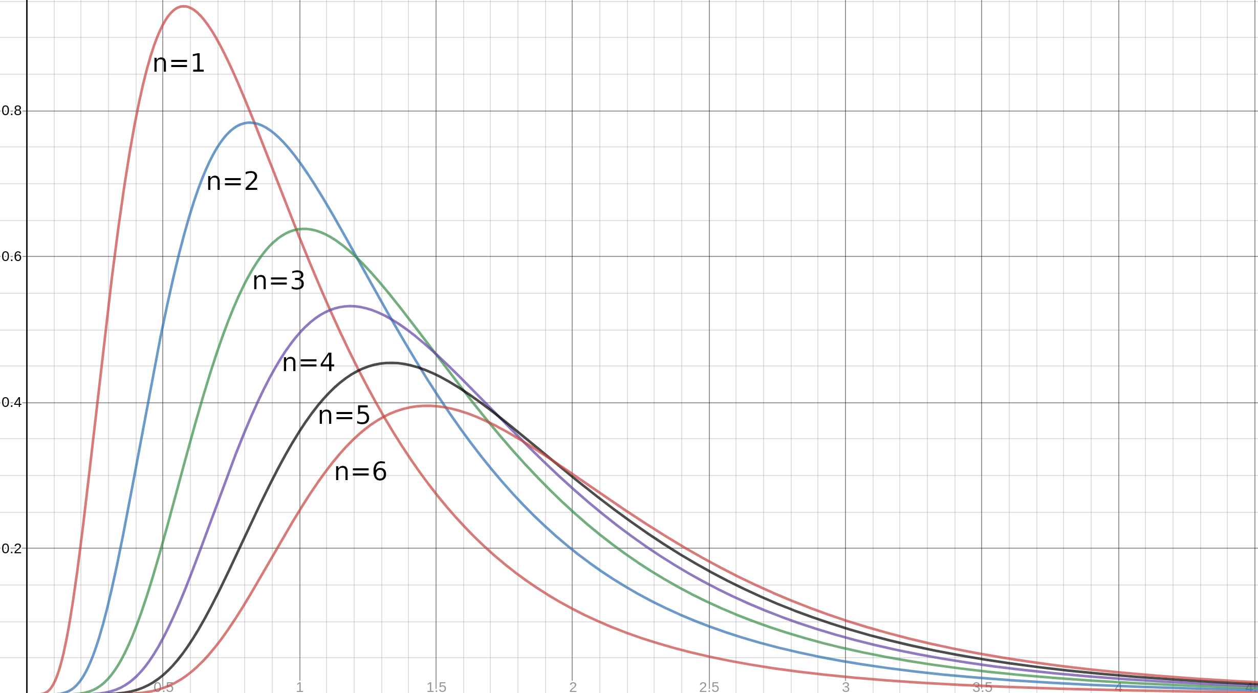
And numerically integrating gets us definite numbers.
| n | Winning Bid | Overpay % | 1 Year Return |
|---|---|---|---|
| 1 | 1.00 | 0% | 88% |
| 2 | 1.34 | 34% | 40% |
| 3 | 1.56 | 56% | 21% |
| 4 | 1.72 | 72% | 9% |
| 5 | 1.85 | 85% | 2% |
| 6 | 1.96 | 96% | -4% |
| 7 | 2.06 | 106% | -10% |
| 8 | 2.14 | 114% | -14% |
| 9 | 2.22 | 122% | -18% |
| 10 | 2.28 | 128% | -22% |
The row n=1 shows the results if you are the only bidder. The expected winning bid is in the “Winning Bid” column. We assume that the winning bid when n=1 is the “correct” price, as discussed. As the number of bidders increases so does the expected winning bid, as we conjectured. The “Overpay %” column shows the ratio of the expected value of the winning bid in that row to the “correct” price, less one. This is the how much more than the correct bid the winner paid. The “1 Year Return” column shows the expected return to that bid after one year. When there is only one bidder the expected return is 88% per year (if this didn’t equal Cochrane’s number the math would be wrong, of course, but always a useful sanity check) but the expected return drops sharply as more bidders enter the auction.
The upshot is that the more bidders on a deal, the lower the expected return of the winner. Given Cochrane’s numbers, if there are more than five bidders, the winner will probably lose money in the first year. But even if there are only two, the expected return is less than half what each bidder had aimed for. Again, this is not a supply and demand issue, it arises from inaccuracies in estimating the correct price. You do not have a lower return because you have decided to bid higher, you have a lower return because only your bids that are mistakenly too high get accepted. Since your bids that are mistakenly too low are not accepted, the resulting pattern of accepted bids is no longer symmetric around the return you had hoped for.
Is there anything you can you do about it?
The best solution is to make sure you have all available information before bidding. This lowers your variance so your bids cluster more tightly around the correct bid. It doesn’t mean you’ll always win–others may overpay–and to the extent that there is still some variance in your bids you will stil not hit your target return, but the effect will be lessened. Do your due diligence.
The problem is that I assume you are already doing your due diligence. But due diligence is not just finding all available information about the company, it’s also having all available information about their market, and adjacent markets, and the markets of their customers and suppliers, and of companies that may decide to enter the market, and of the technology, and competing technologies, and nascent technologies, etc. It’s a lot of information. You can do better, always, but you can never really be close to perfect.
You could also always bid low to compensate for this effect. This is what economists think would happen. There are a few difficulties doing this:
- Your bid is as accurate as you can make it, so you may feel that bidding low is irrational;
- Other bidders may not adjust their bids, so you may end up losing auctions that would have given you good returns–and even auctions where the winner gets good returns (though on average that winner would not get good returns);
- Compensating the bid would require knowing how many other bids there will be–no smart founder will tell you this.
I have never heard of a VC adjusting their bid downwards because they believe there will be many other bidders; usually the opposite happens. If this is so, then the second point, above, would be even more acute. You could end up losing every auction and never doing a deal. This might be a worse result for you than low returns. At least in an environment where multiple bids (and, therefore, overpaying) are the norm you wouldn’t be underperforming your peers. As Chuck Prince said, as he was helping to almost destroy the world financial system: “when the music is playing, you’ve got to get up and dance.”
Or, you can refuse to bid if there are other bidders. But because you would have to do this on every deal (since you can’t know on any given deal if you are bidding erroneously high or low) it is entirely impractical. Not least because founders, as mentioned, will not let you know you’re the only bidder. You might be able to avoid bidding on companies that look like they’ll have many term-sheets…when companies are going to get three or more bids, say, it is often fairly evident. Keeping n<3 will do a lot to improve your overall returns.
[Update: Tom Loverro pointed out another way to do this–preemptively bid on follow-on rounds. This dramatically lowers the probability of other bidders. He says he has noticed this occurring more frequently recently, and so have I. One explanation is that VCs are already noticing and trying to avoid the cost of winning.]
This, of course, is common wisdom. Be a contrarian. Climb the wall of worry. Buy low, sell high.
But cliches are cliches because there is some grain of truth. The truth here is that no matter how disciplined you are, you will have lower returns when there are many bidders. The only way to avoid paying the cost of winning is to avoid situations where there are many bidders: both specific deals where there is a feeding frenzy and entire time periods when there are too many bidders in the market.
This last point has a bit of a twist. Supply and demand can drive prices higher when there is too much money in VC.6 But the cost of winning is driven up when there are too many bidders, independent of how much money each has. In a time period, like today, when there are many more seed-stage funds than there have historically been, it’s inevitable that the average number of bidders on each deal will increase. Because the returns decline steeply with even a small increase in bidders–from one to two or from two to three–we should expect that in this fragmented market most VCs who win early stage deals will have heavily overpaid. We talk a lot about the obvious problem of too much money in venture, less about what may be an even bigger drag on returns, fragmentation.
Caveats:
- I have assumed that Cochrane’s mean returns are the mean returns if there is one bidder. Most venture rounds only have one termsheet, especially at the first round and especially over a longer period of time, as Cochrane’s data is, so this is not entirely inaccurate. But it is almost certainly true that the average number of bids on a given venture round is higher than one, even if only fractionally so, so the mean return should be shifted to that number of bidders and all the other numbers recalculated. I have not done this since I think the effect is small and I don’t know the actual average number of bidders over the time period of Cochrane’s data.
- These numbers assume that bidders did not correct their bids to account for the cost of winning.
Thank you to Abhishek Ranjan who straightened me out on mean log returns and variance log returns.
Let me just define what I mean by “correct” price here: this is the price at which I expect to get my target IRR. For instance, if the expected value of the equity I am buying in the startup is $20m in 10 years and I want a 40% IRR, then the value of the equity today is $20m/1.4^10. This is the correct price. It does not mean that each and every company I back will achieve its expected value, natch. ↩
Cochrane, JH. “The Risk And Return Of Venture Capital,” Journal of Financial Economics, 2005, v75, pp. 3-52. ↩
This method is described in detail all over the place. See for instance: http://pages.stern.nyu.edu/~adamodar/pdfiles/valn2ed/ch23b.pdf ↩
This excludes things like preferences, cost of capital, etc. But because venture capital firms are almost entirely homogeneous other than in the information they have, I feel comfortable with this simplification. ↩
Chua Chow, C. & Sarin, R.K., “Known, Unknown, and Unknowable Uncertainties”, Theory and Decision (2002) 52: 127. https://doi.org/10.1023/A:1015544715608 ↩
History seems to show that the best IRRs are achieved by funds started in years when VC is out of favor. ↩